


GLMM Methodology
The modeling of individual longitudinal data may be approached in a quite intuitive way:
1. Traditional way: Multiple linear regression ![]()
Individual curves, from multiple linear regression of ln(PSA) on time, only observed 'within a given patient'. These curves would then be averaged in some way and a "reference" PSA evolution derived. The corresponding individual PSA DT is calculated as ln2/λ (Choo et al., 2004). The average DT would be estimated by individual DTs with large range.
2. Better approach: General linear mixed model ![]()
Longitudinal data observed in a set of patients are advantageously analyzed by the "general linear mixed model (GLMM)" (Laird and Ware 1981; Verbeke and Molenberghs, 1997). The GLMM includes fixed (Xiβ) and random (Ziγi) effects (random intercept and slopes), and allows for individual predictors of intercept and slope to be integrated into model. εi is a vector of residual components specific to the subject. Individual or average PSA DT would be calculated by GLMM with a small range. An average (reference) PSA evolution could be derived as well.
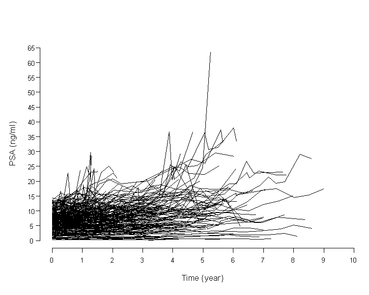
For example, the following figure shows that serial PSA measurements over time in actual 231 patients. Each individual has his own intercept and slope. Between variability (8.2 with a range of 0.09-63.6) is larger than within variability (2.1 with a range of 0.05-14.3), both of them have wide range. This model observed either 'within a given patient' or 'between different patients'. Thus, the GLMM approach goes beyond classical multiple regression analysis.
The GLMM was fitted by the SAS Mixed procedure (version 9.1). Akaike's Information Criterion was used for comparing models AIC = LREM + 2 * k, where LREM represents the restricted maximized -2(log likelihood) of the fitted model and k the number of parameters in the model. The lower the AIC, the better the model. Receiver Operating Characteristics (ROC) curve analysis was used to compare the distributions of observed points (%) for patients in high risk and low risk groups. The area under the curve (AUC), sensitivity, specificity and overall accuracy were also applied. Results were considered significant at the 5% critical level (p < 0.05).
